Excel 2010, released in 2010, introduced several notable new features and improvements compared to previous versions. Here are some of the new features in Excel 2010:
Nội dung
1. Backstage View
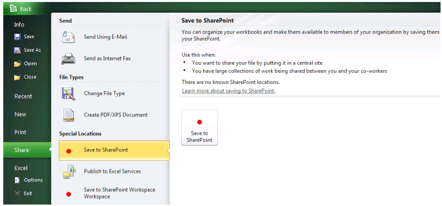
All applications within the Office 2010 suite are equipped with the Office 2010 Ribbon interface. The Backstage View tool, accessed via the Office button in the upper left corner of the screen, allows users to perform tasks such as saving documents (Save) and printing (Print). Additionally, the left navigation pane contains many commands, such as: Allowing others to edit documents or adjusting file sizes:

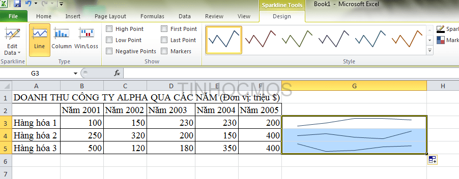
2. Sparklines
Excel has always been used as a powerful tool for describing trends and data through rich graphs and charts. With the 2010 version, the new Sparkline feature allows users to place a small graph or a trendline in a cell. With various chart types (column, line, win/loss) and pre-set color combinations in Excel, Sparklines are an effective tool for faster data analysis and orientation to provide a simpler view when observing information and making decisions.

3. Slicers
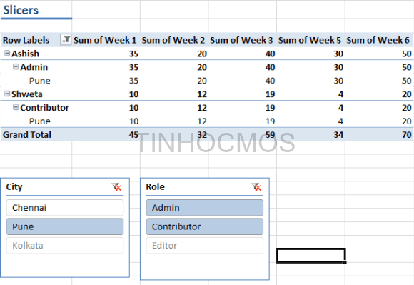
In Excel 2010, slicers are added as a new way to filter PivotTable data. Through this tool, you can quickly get a deep visual view of a large amount of data.

When the data in the PivotTable changes, Slicers are automatically updated, providing convenience for users.
4. Conditional Formatting
One of the most useful new features of Excel 2010 is Conditional Formatting—a feature that includes many formatting styles and icons and the ability to highlight only specific items such as the largest or smallest values with just one click. With this feature, instead of using functions to extract and filter data from a table containing various numbers, you can still accurately evaluate the data by highlighting cells based on predefined conditions. Here’s how to do it: select a column or row of data to evaluate, then click the Conditional Formatting button. A menu will appear with options:
Filter-based evaluation types:
This evaluation type filters your data directly within the table rather than extracting it as in earlier versions of Excel. The program performs “in-place filtering” by highlighting cells that meet the conditions or rules you define. Below are two main rule groups:
Highlight Cells Rules:
Highlights cells based on one of the following conditions:
- Greater Than…: Greater than a specific value.
- Less Than…: Less than a specific value.
- Equal To: Equal to a comparison value.
- Between: Between two specified values.
- Text that Contains: Contains specific text.
- A Date Occurring: Matches a date range.
- Duplicate Values: Highlights duplicate values.
After selecting a highlighting condition, a dialog box will prompt you to enter the value to compare and the highlight color for cells matching the condition. Click OK to apply the formatting to your table.
Top/Bottom Rules: This rule group includes the following conditions:
- Top 10 Items: Highlights the 10 cells with the highest values.
- Top 10%: Highlights the top 10% of cells with the highest values.
- Similarly, Bottom 10 Items and Bottom 10% highlight the lowest values.
- Above Average: Highlights cells with values above the column/row average.
- Below Average: Highlights cells with values below the column/row average.
When using Top or Bottom data evaluations, a dialog box will prompt you to input the number of cells to highlight, such as the top 10 or 20, top 10% or 20%, etc., allowing for adjustments. Click OK to finalize.
Display level evaluation types:
Data Bars: Select this type of evaluation and choose a preferred color from the menu. A color bar will appear in your data range, providing a visual representation of data levels, helping you quickly identify increases or decreases. The longer the color bar, the higher the data value, and vice versa for lower values.
Color Scales: This evaluation type colors data cells with three different shades, corresponding to low, medium, and high levels. When choosing the Color Scales group, select a preferred color scheme from the menu, and the program will apply it to your selected range. You can also create custom rules by selecting Color Scales > More Rules.
Icon Sets: Select Icon Sets and choose a desired icon group. The program will automatically place icons in front of your data cells, providing a visual representation of the data table.
For instance, one icon indicates the highest data level, another represents the average level, and another signals below-average levels, raising an alarm. Each icon corresponds to a specific level, with the program calculating the average value of the column or row and assigning icons to cells based on their percentage compared to the overall range.
You can redefine these evaluation rules by selecting More Rules in the Icon Sets group.
Custom Conditional Formatting Rules:
In addition to the above predefined conditional formatting options, you can create your own evaluation rules by clicking Conditional Formatting > New Rule. However, this can be time-consuming. It’s usually best to leverage the existing, comprehensive rules Excel provides.
If you’re not satisfied with the applied formatting, you can remove it without losing data by clicking Conditional Formatting > Clear Rules and selecting an option:
- Clear Rules from Selected Cells: Removes formatting from the selected range.
- Entire Sheet: Clears formatting from the entire sheet.
- This Table: Clears formatting within the currently processed table.
5. PivotTable and PivotChart
In Excel 2010, when creating a PivotChart, special PivotChart tools and context menus are provided so you can analyze data in the chart. You can also change the layout, style, and formatting of the chart or other components of it in the same way you can do for regular charts. The chart formatting you apply is maintained when switching to PivotChart, which is an upgrade addition to the way it worked in previous versions of Excel.
SharePoint is integrated into Excel 2010, providing easy-to-understand content management tools for sharing knowledge, enhancing teamwork, and productivity.

The new features of Excel 2010 have improved over previous versions. It helps to work more efficiently and creatively, especially in data analysis and management. I hope this article is helpful for you when updating your knowledge about Excel 2010.
See more: How to Get Data from One Table to Another in Excel (Detailed Guide)
