If you want to hide data in Excel but don’t know how this article will help you. In addition to hiding text and values in Excel, you can also hide other things such as rows, columns, and more. Let’s explore together.
Nội dung
1. How to hide overflow text in Excel
When you enter text into a cell, if the text is longer than the cell, it will overflow into the adjacent cells in the row. If the adjacent cell already has text, the text in the first cell will be blocked by the text in the adjacent cell. You can solve this problem by adding text to the first cell, but this will increase the height of the entire row.
If you don’t want to display overflow text even when adjacent cells are empty then hide overflow text in Excel .
- Select the cell containing the overflowed text and follow these steps:
- Right-click on the selected cell(s) and select Format Cells.
- Press Ctrl + 1.
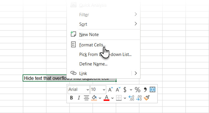
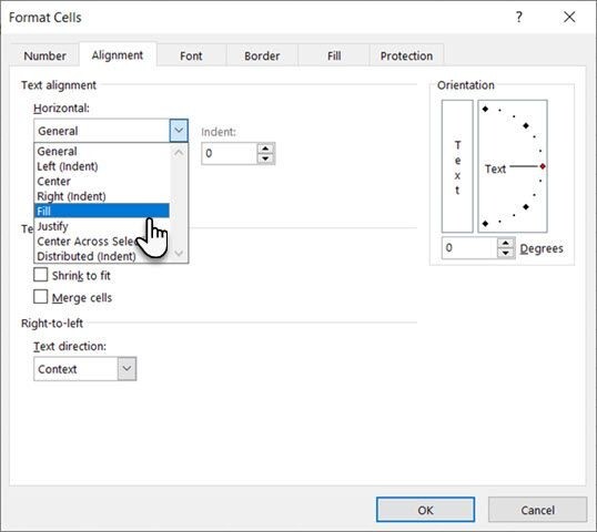
- On the Format Cells dialog box, click the Alignment tab. Then, select Fill from the Horizontal drop-down list, and then click the OK button.
- Overflow text in the first cell is not visible even if the cell to the right is empty.
2. How to hide and show comments in cells
Comments in Excel allow you to annotate your worksheets. This is useful when working with others on a worksheet. You can set reminders or add notes for yourself or others to explain a formula or how to use a part of the worksheet.
You can also hide comments if there are too many comments on your worksheet. Sometimes comments make it difficult to read the data.
By default, cells with comments contain a small triangle in the upper-right corner called the comment indicator. To hide comments, follow these steps:
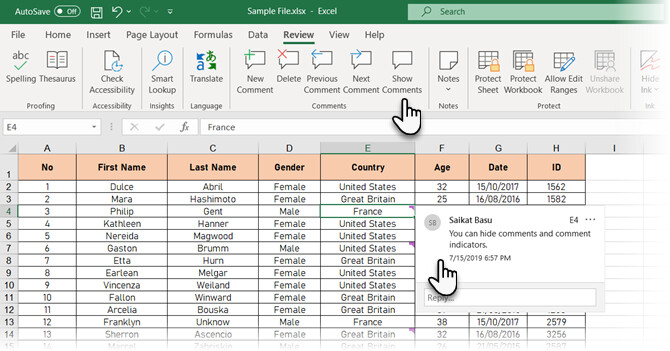
- To hide comments on an individual cell, you need to select that cell and click Show Comments in the Comments section of the Review tab.
- To show comments again, select the same cell and turn the Show Comments button back on.
- To show or hide comments on multiple cells, use the Shift and Ctrl keys to select the cells and toggle the visibility using the Show Comment button.
- To show all comments at once, simply click Show Comments in the Comments group on the Review tab. This option shows all comments on all open workbooks. When this option is on, any workbook you open or create will show all comments until you turn this option off.
Steps to control comment visibility in Excel
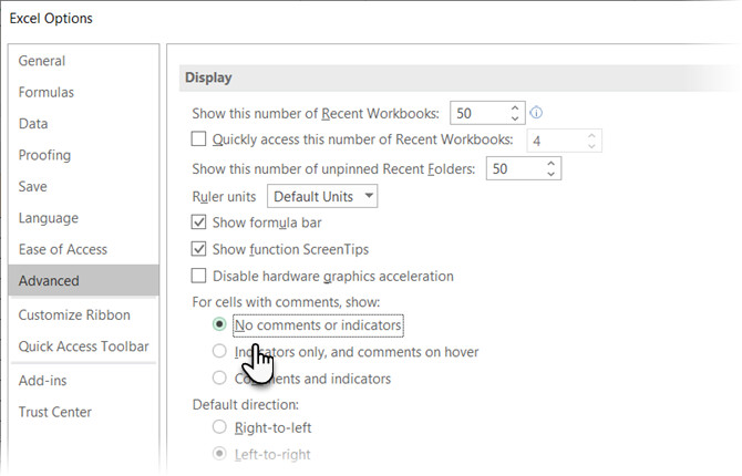
- To hide all comments and comment indicators, go to File > Options.
- Click Advanced on the left, then scroll down on the right to the Display section.
- Select No comments or indicators in For cells with comments, show. Indicators and comments will be hidden and will not appear when you hover over cells.
- To show comments and indicators again, simply select one of the other two options. Or click Show All Comments in the Comments section of the Review tab.
- The options in For cells with comments, show in the Excel Options section, and Show All Comments on the Review tab are linked together.
Commenting is essential for effective collaboration, so make sure you understand all the ways to manage comments in Excel if you share a workbook with a team.
3. How to hide and show certain cells
You can’t hide cells themselves, but you can hide cell contents in Excel. For example, you have some data that is referenced by other cells but you don’t need it.
To hide the contents of a cell, select the cell(s) you want to hide (use the Shift and Ctrl keys to select multiple cells). Then, do the following:
- Right-click the selected cell(s) and select Format Cells.
- Press the shortcut Ctrl + 1.
- On the Format Cells dialog box, you need to turn on the Number tab. Then select Custom in the Category box.
- Before changing the Type, double-check what you’ve selected to see what will change it back when you redisplay the content.
- Enter three semicolons (;;;) in the Type box and click the OK button.
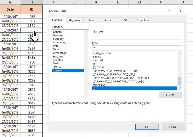
The contents of the selected cells are now hidden, but the value, formula, or function in each cell is still visible in the Formula Bar .
Hidden content is still available for you to use in formulas and functions in other cells. If you replace the content in a hidden cell, the new content will also be hidden. The new content is available for use in other cells just like the original content.
To display the cell contents again, simply follow the same steps above. But this time, select the Category and Type for the cells on the Format Cells dialog box.
4. How to hide and show the formula bar
Even if you hide a cell, its contents, formula, or function will still be visible in the Formula Bar. To completely hide the contents of a cell, you must also hide the Formula Bar.
On the View tab, clear the Formula Bar check box in the Show section.
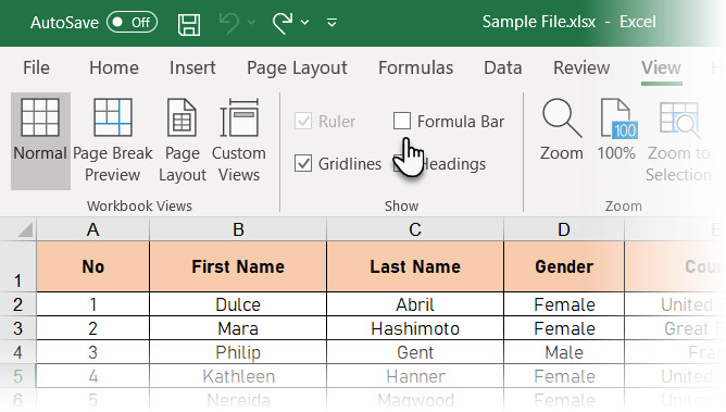
You can also hide the Formula Bar on the Excel Options dialog box.
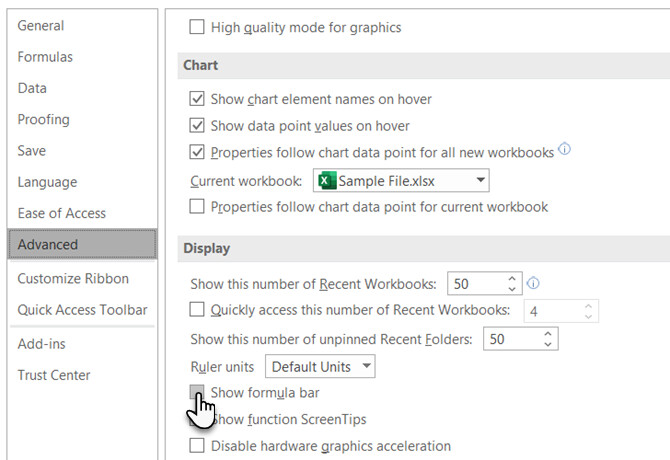
Go to File > Options. Then, click Advanced on the left and uncheck the Show formula bar box in the Display section on the right.
5. How to hide and show formula contents in cells
By default, when you enter a formula in a cell, the formula displays in the Formula Bar and the result displays in the cell.
If you don’t want others to see your formulas, hide them. The first way is to hide the Formula Bar as in the previous section. However, this method is not very effective because anyone can show the Formula Bar again.
Another, much more effective way to hide formulas is to apply the Hidden setting to the cell and protect the worksheet.
- Select the cell(s) you want to hide the formula(s) for and do the following:
- Right-click the selected cell(s) and select Format Cells.
- Press the shortcut Ctrl + 1.
- On the Protection tab, check the Hidden box. Then click the OK button.
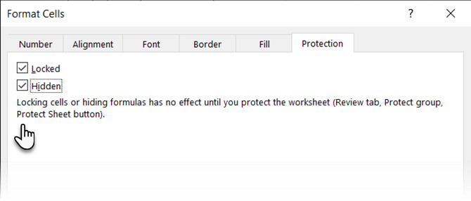
You still need to protect the worksheet to hide the formulas by selecting Protect Sheet in the Protect section on the Review tab.
In the Protect Sheet dialog box, check the Protect worksheet and contents of locked cells box.
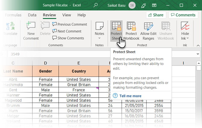
In the Password to unprotect sheet box, enter a password to prevent others from unprotecting the sheet. This is not required, but we recommend that you do so.
By default, Select locked cells and Select unlocked cells are selected in the Allow all users of this worksheet to box. You should not select any other actions if you do not want other users to change your worksheet.
Re-enter your password in the Confirm Password dialog box.
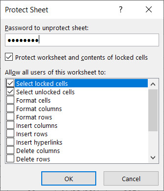
The formulas in the selected cells won’t be visible in the Formula Bar, but you’ll still see the results of the formulas in the cells, unless you’ve hidden the contents of those cells as described in the “How to hide and unhide some cells” section above.
To show formulas again, select the cells you want to show formulas for and click Unprotect Sheet in the Protect section of the Review tab.
If you entered a password to protect the worksheet, you need to re-enter the password in the Unprotect Sheet dialog box to display the formulas.
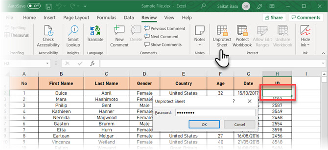
The formulas won’t be visible. Reverse the process you did to hide the cell contents and turn off the Hidden setting for them.
- Select the cells whose formulas you have hidden and do the following:
- Right-click the selected cell(s) and select Format Cells.
- Press the shortcut Ctrl + 1.
- Uncheck the Hidden box on the Protection tab and click the OK button.
The formulas of the selected cells will reappear in the Formula Bar if you have not hidden the Formula Bar.
6. How to hide and show rows and columns in Excel
If you don’t use one or more rows or columns in your worksheet, hide them. The process of hiding and showing rows and columns is almost the same as above, except for the keyboard shortcuts.
Hide and show rows in Excel
To hide one or more consecutive rows, first select the rows. Then, do the following:
- Right click on the selected rows and select Hide.
- Press the shortcut Ctrl + 9.
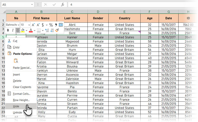
Selected rows are replaced with a double line in the row header and a bolder line in their location. When you click anywhere on the worksheet, this bold line disappears, but you can still tell where the hidden rows are by the missing row number and the double line in the row header.
Cells in hidden rows and columns are still used for calculations while hidden.
The quickest way to show a single row. Hover over the hidden row marker. When the mouse pointer turns into a split double-headed arrow, double-click it.
Or use the shortcut key: Ctrl + Shift + 9
To show specific adjacent rows. Select the rows above and below the hidden rows. Then, do the following:
- Right click on the selected rows and select Unhide.
- Press the shortcut key Ctrl + Shift + 9.
Show all rows in the worksheet. Click the Select All button (the small triangle at the intersection of the row and column in the upper right).
- Right click and select Unhide.
- Press the shortcut key Ctrl + Shift + 9.
This unhide method does not work on the first row of the worksheet because there is no row above the first row. There are also some other bugs that make Excel hidden cells unable to unhide .
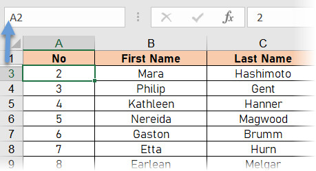
To select the first row, click the Name box on the left side of the Formula Bar, type “A1” if the hidden row is the topmost in the worksheet, or “A2” if you’re using column headers as shown in the screenshot below. Press Enter. Then press Ctrl + Shift + 9.
Hide and show columns in Excel
The hiding options in Excel for similar rows and columns are the same. Select the column or consecutive columns you want to hide and do the following:
- Right-click the selected columns and select Hide.
- Press Ctrl + 0 (zero).
The same double and bold lines you see when you hide rows will appear where columns are hidden. The column letters are also hidden.
To show columns again, select the columns to the left and right of the hidden columns. Then, do the following:
- Right click on the selected columns and select Unhide.
- Press the key combination Ctrl + Shift + 0 (zero).
If you have hidden the first column (A) then you can display it as if you had hidden the first row.
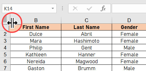
The quickest way is to drag the colored line to the right and reveal the first hidden row. Hover over the marker as shown in the screenshot below until the mouse pointer changes to a split double-headed arrow. Then drag to the right.
To select the first column, click the Name box on the left side of the Formula Bar, type “A1” and press Enter. Then, press Ctrl + Shift + 0 (zero).
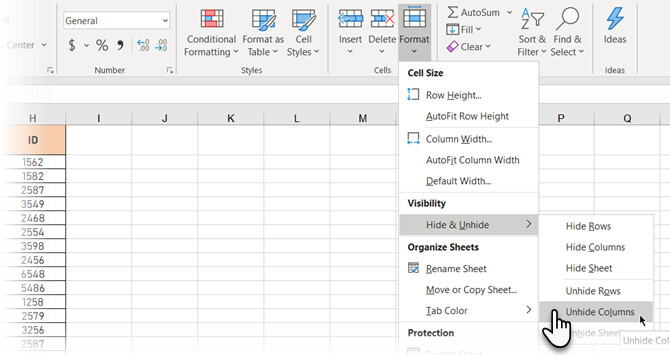
There are some cases where the show shortcut doesn’t work. Instead of using the shortcut, type “A1” and press Enter to select the hidden column. Then, go to Home > Cells Group > Format > Visibility > Hide & Unhide > Unhide Columns.
If you have hidden multiple rows and columns, you can show all hidden columns at once.
- Select the entire spreadsheet by clicking the box between the row and column headers or pressing the keyboard shortcut Ctrl + A.
- Then press Ctrl + Shift + 0 (zero) to show all hidden columns.
- Another way is to right-click on the row or column header while selecting the entire worksheet and select Unhide.
Hiding data is a simple yet extremely useful Excel skill. I hope this article helps with your work. Wishing you success.
See more: The simplest way to convert columns to rows in Excel
