Detailed instructions on how to use Filter data in Excel

1

Filter in Excel is a very useful tool and indispensable for those who often use Excel. In this Excel lesson , we will learn how to use filters in Excel to see its effects clearly. You will know how to use filters to filter data in Excel with Text (text), Number (number) and Date/Time (Date, time) formats.

1. How to create a filter in Excel

Filter in Excel, also known as Filter (or AutoFiltter), is a tool that helps you search, filter data, and sort data… so that you can more easily manage data. You can create a filter by:

Step 1: select the entire data table, from the title row to the last row with data in the table (or you can select more blank rows below)

Step 2: on the Data tab on the toolbar, click on the Filter function

Sau khi chọn Filter, trong bảng dữ liệu sẽ xuất hiện biểu tượng hình mũi tên hướng xuống dưới tại dòng tiêu đề. Đây chính là biểu tượng của bộ lọc.

Attention

Some things to keep in mind when creating filters are:

1. You can quickly create a filter by selecting any position in the table and then selecting Filter on the Data tab. Excel will automatically understand that you want to apply the filter to the spreadsheet containing the position you are selecting. However, sometimes Excel misunderstands because your table structure is not up to standard, leading to incorrect filter application. You should select the entire table instead of just selecting 1 position in the table.
2. Filters sometimes break at blank rows in a table. Blank rows mean that there are no cells containing data on the entire row.
3. If the spreadsheet has merged cells in the header row, the filter will apply to the first (top) row and not the bottom row in the header area.
4. Filters appear only in the header row (usually the first row at the top of a table). If there is no separate header row, Excel assumes the first row in the table is the header row.

2. How to use filters to manage data

Filters have many uses, not just filtering data. Let’s learn the main functions of filters:

Sort data in a spreadsheet using Filter

When you click on the filter symbol in the data table, you can see that the filter has a Sort function right at the first part. There are 2 ways to sort:

• Sort A to Z is to sort from A to Z (in ascending order)
• Sort Z to A is to sort from Z to A (in descending order)

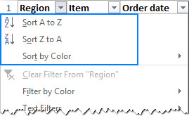
The sorting in Filter has the following feature: only the displayed values ​​are sorted, while the hidden values ​​(filtered out because they do not match the filter conditions) are not sorted. This is very different from using the separate sorting function on the Data tab.

Filter operations

When a down arrow icon  appears in the title line, it means that the filter has been added, but is not yet being applied (or is not filtering based on any conditions).

To filter data in Excel, follow these steps:

1. Click the down arrow on the column you want to filter.
2. Uncheck Select All to quickly remove all objects.
3. Select the object you want to filter for, and then click OK.

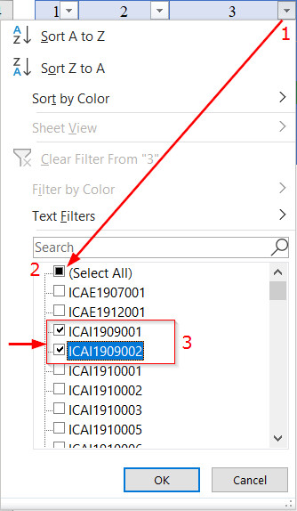
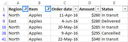
After filtering, the down arrow icon in the filtered column changes to a funnel icon, indicating that a filter is being applied to the column.

Characteristics of the data table when in filter mode:

• There is a funnel icon on the filter in the subject line
• The Heading section displays the number of rows in blue (usually black) and has hidden rows (values ​​that do not match the filter conditions).
• The remaining columns in the table will only have content corresponding to the row containing the value that satisfies the previously applied filter condition.

You can filter multiple columns at once instead of just filtering one column. Then the funnel icon can appear on multiple columns at once:

How to expand the information panel in the filter

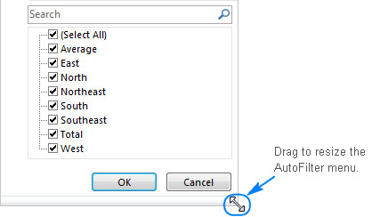
In addition, you can control the filter window in Excel to become wider, displaying more content by moving the mouse to the lower right corner of the table area when opening the filter, and as soon as the double-headed arrow icon appears, hold the mouse and drag it down or drag it to the right, the filter information table will expand in the corresponding direction.

How to filter out blank cells in a table

To check if there are blank cells in your column, you can click on the filter button icon on the header row and pay attention to the bottom of the filter objects: If the item (Blanks) appears, it means there are blank cells.

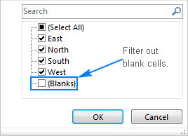
• You can uncheck this box to filter out blank cells in the column you want to filter, then click the OK button.
• Alternatively, you can click to remove the checkmark in Select All, then select Blanks only to display only blank cells.

How to filter text data

For columns containing text data, when you click on the filter, you will see the Text Filters line appear. Then you can use the filter conditions applied to text data (Text).

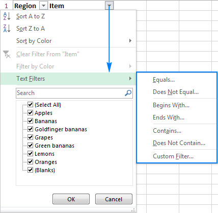
For example, to filter out rows that contain Bananas, do the following:

1. Click the down arrow in the column header, and then select Text Filters.
2. In the Text Filters filter criteria, you can select the Does Not Contain item.
3. The Custom AutoFilter dialog box will appear. You can enter the content you want to filter out, then click OK.

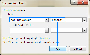
As a result, all rows containing the character bananas, including Bananas, Goldfinger bananas, Green bananas are hidden from the data table.

Filter by 2 conditions on the same column

To filter data in Excel with more than 1 condition, you can select the Custome Filter item (the bottom line in the list of filter criteria in the Text Filter selection panel). The Custom AutoFilter panel will then appear and you continue to perform the following operations:

1. Select the first filter condition including the operator (words that represent a range of values ​​such as Contains, Does not contain…) on the left side and the value of the accompanying condition (on the right side)
2. Choose whether the relationship between these conditions is And (both true) or Or (only one case needs to be true)
3. Select the comparison operator and the value of the second condition.

For example, we will filter for either bananas or lemons, then set it up like this:

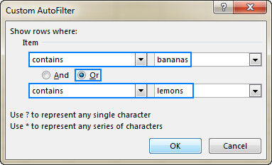
Then the filter result is that the rows with the value banana or lemon appear, otherwise these two values ​​will be hidden.

How to filter data by wildcard characters

If you have a lot of Text data and you don’t remember exactly what you want to filter, you can use wildcards:

• The asterisk character * represents any character, with no limit on the number of characters.
• The ? character represents any character, with a limit of 1.

How to filter data in Number format in Excel

Similar to text format, if the column contains data that is numbers, the filter in Excel will automatically change, not Text Filters but Number Filters. That is, the filtering method will change based on the type of data in the column to be filtered.

The characteristic of Number data is that it is automatically sorted in the filter in ascending order (including negative numbers and decimal numbers).

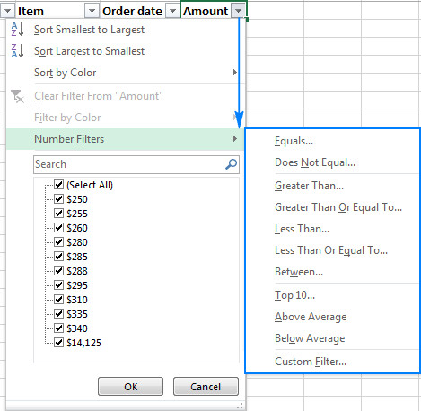
For example, to filter values ​​from 250 to 300, we can select Between and set it as follows:

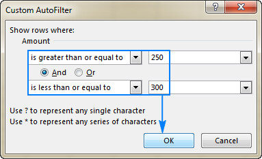
in there:

• is greater than or equal to means greater than or equal to (from how much)
• is less than or equal to means less than or equal to (to how much)

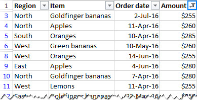
As a result, only orders with a value between $250 and $300 are displayed.

Filter data by time in Excel

First of all, you need to pay attention that we encounter many errors in time data. Specifically:

• Normally when writing (or entering) time values ​​in Excel, we implicitly understand that we will enter the previous day, next month, and then the year.
• But Excel has a default setting that understands that users will enter the format Month First, Day Next, then Year.

Such different understandings lead to incorrect time values ​​you enter, causing the filtering results to not be as expected. You need to know how to format Date Month Year in Excel correctly to make sure the data is not incorrect.

The characteristics of time data are:

• Show Date Filters item in the filter
• Automatically group by Year > Month > Day in the filter content table

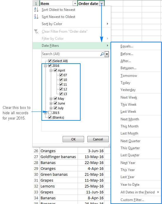
You can use the filter methods according to the conditions provided in Date Filter very quickly and appropriately to your needs. Or you can use Custom Filter to enter the desired value.

How to filter data by color in Excel

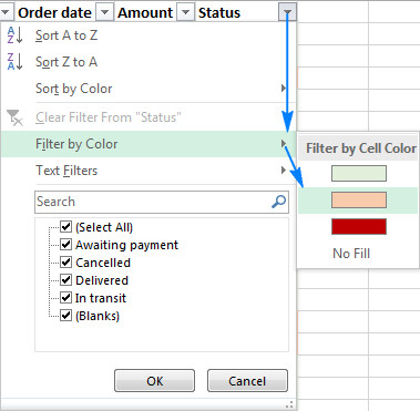
In addition to filtering by specific values, Excel lets you filter by colors formatted in cells, including:

• Background color in cell
• Text color in cell

When you use the direct coloring method or use Conditional formatting to automatically change colors according to conditions , you just need to use the available colors to filter for suitable values:

How to reuse filters when data is updated

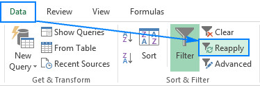
When data is updated (added / changed / deleted …) the filter results will be different. Therefore, you will need to update the filter results again. There is a very simple way, which is to use the Reapply function on the Data tab. Here’s how:

Applicable conditions: When you are applying a conditional filter (filtering state).

On the Data tab, click on the Reapply position (as shown below), it means Reapply the filter condition to update the results. This function is shown below:

or:

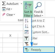
You select the Sort & Filter tool on the Home tab > Select the Reapply item

How to copy filter results to another location

After filtering data in Excel, you may need to copy the filtered results to another location, such as another sheet or another workbook. Here’s how:

1. Select the data area to copy. Note that this area only contains results that match the filter conditions.
2. Right-click and select Copy (or press the shortcut key Ctrl + C) to execute the copy command.
3. At the place where you want to paste the filter results, click on the first cell in the area where you want to paste the results, right-click and select Paste (or press the shortcut key Ctrl + V).

Some notes when copying filter results

Normally, when copying filtered data to another location, using the above operation, you will get the remaining values ​​after filtering.

But in some cases Excel displays the entire content, including hidden (filtered) values. To fix this problem you can do the following (starting after step 1 of the 3 steps above)

Method 1: Press Alt +; to select only the visible cells. Then Copy.

Method 2: Press the F5 key on the keyboard to open the Go To… window. Then select Special… > In the Goto Special window, select Visible Cells only (only visible cells). Then copy this data.

How to remove filters or filter results when you don’t want to use them

When you want to return to the state before filtering, or want to remove the filter from the data table completely, you can use the following operation:

1. To clear the filter condition , click on the filter in the column being filtered, select Clear Filter as shown below:

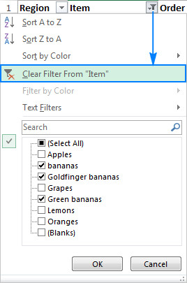
Or you can go to the Data tab > Sort & Filter group, then select Clear.

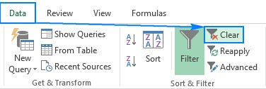
2. To remove the filter, click the Filter icon again in the Data tab. It now acts as a switch, the active state is surrounded by green around the Filter icon, when you click it again, the green color disappears and returns to normal. At that time, the filter will no longer appear on the data table.

Hopefully, this article will be useful in improving your Excel skills. If you have any questions, you can comment and respond right below this article so that we can resolve all your questions as soon as possible.

See more: Automatically draw cells in Excel