Nội dung
1. Time format in Excel
If you’ve followed our Excel Dates tutorial, you’ll know that Microsoft Excel stores dates as sequential numbers starting from January 1, 1900, as the number 1. Because Excel treats times as a fraction of a day, times are stored as decimal fractions.
In Excel’s internal system:
- 00:00:00 is stored as 0.0
- 23:59:59 is stored as 0.99999
- 06:00 am is 0.25
- 12:00 PM is 0.5
When both a date and a time are entered in a cell, they are stored as a decimal number consisting of an integer part (representing the date) and a decimal part (representing the time). For example, June 1, 2015 9:30:00 AM is stored as 42156.3958333333.
2. Quick way to get a decimal representation in Excel
A quick way to select a decimal number that represents a specific time is to use the Format Cells dialog box.
It’s pretty simple. Just select a cell containing the time and press Ctrl + 1 to open the Format Cells dialog box. On the Number tab, select General under Category, and you’ll see decimals in the Samples box.
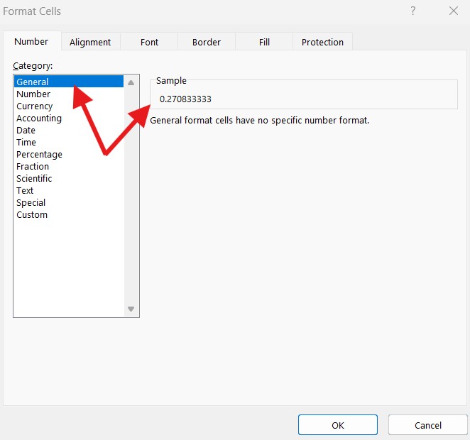
Now, you can write down the number you get and click Cancel to close the window. Or, you can click the OK button and have the time replaced with the corresponding decimal number in the cell. In fact, you can think of it as the fastest, easiest, and formula-free way to convert time to decimal in Excel. However, we will introduce it in the next part of this article, and then we will take a closer look at the special time functions and calculations that can convert time to hours, minutes, or seconds.
3. How to apply or change time format in Excel
Microsoft Excel is smart enough to recognize a time when you enter it and format the cells accordingly. For example, if you enter 20:30, or 8:30 PM, or even 8:30 in a cell, Excel will interpret this as a time and display it as 20:30 or 8:30, depending on the default time you have formatted.
If you want to format some numbers as times or apply a different time format to the current time value, you can do this using the Format Cells dialog box, as shown below.
In an Excel sheet, select the cell(s) to which you want to apply or change the time format.
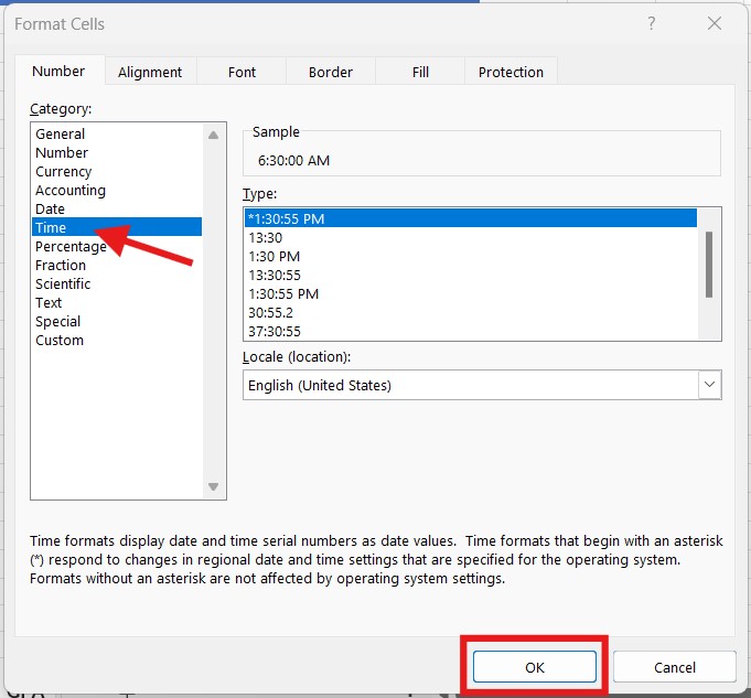
Step 1: Open the Format Cells dialog box by pressing Ctrl + 1 or clicking the Dialog Box Launcher icon next to Number in the Number group , on the Home tab .
Step 2: On the Number tab , select Time from the Category list and select the desired time format from the Type list .
Step 3: Click OK to apply the selected time format and close the dialog box.
3. 1 Create a custom time format in Excel:
Although Microsoft Excel provides a limited number of different time formats, sometimes you want to create your own format that best suits a particular worksheet. To do this, open the Format Cells dialog box , select Custom from the Category list , and type the time format you want to apply in the Type box.
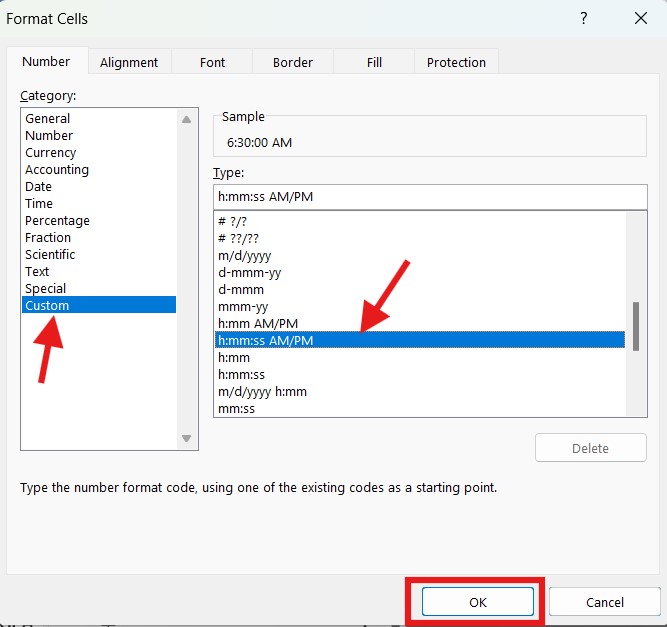
The custom time format you created will be in the Type field and displayed from the next time you use it.
Tip: The easiest way to create a custom time format in Excel is to use one of the existing formats as a starting point. For that, you have to click Time under Category and select one of the predefined formats under Type . Then switch to Custom and make changes to the format shown in the Type box.
When creating a custom time format in Excel, you can use the following codes.
| Code | Describe | To display |
| h | Hour without leading zero | 0-23 |
| hh | 2 digit hour | 00-23 |
| m | Minutes without leading zero | 0-59 |
| mm | 2-digit minutes | 00-59 |
| s | Number of seconds without leading zero | 0-59 |
| ss | 2-digit seconds | 00-59 |
| AM/PM | Time of day (if not formatted, defaults to 24 hour format) | AM or PM |
Tip: To create custom formats for dates and times, use and combine time codes and date codes intelligently.
The following table provides a few examples of how your Excel time formats:
| Format | To display |
| h:mm:ss AM/PM | 1:30:00 PM |
| h:mm | 13:30 |
| dddd, m/d/yy h:mm AM/PM | Tuesday, 1/13/15 1:30 PM |
| ddd, mmmm dd, yyyy hh:mm:ss | Tue, January 13, 2015 1:30:00 PM |
3.2 Custom formats for time periods over 24 hours
When you calculate time in Excel, a cell that contains a total amount of time might exceed 24 hours. To have Microsoft Excel display times beyond 24 hours correctly, apply one of the following custom time formats.
| Format | Display | Explain |
| [h]:mm | 41:30 | 41 hours and 30 minutes |
| [h]:mm:ss | 41:30:10 | 41 hours and 30 minutes and 10 seconds |
| [h] “hours”, mm “minutes”, ss “seconds” | 40 hours, 30 minutes, 10 seconds | |
| d h:mm:ss | 1 17:30:10 | 1 day, 17 hours, 30 minutes and 10 seconds |
| d “day” h:mm:ss | 1 day 17:30:10 | |
| d “day,” h “hours,” m “minutes and” s “seconds” | 1 day, 17 hours, 30 minutes and 10 seconds |
3.3 Custom time format for negative time values:
The custom time formats discussed above only work with positive values. So if your calculation result is a negative value (formatted as a time) (for example, when you subtract a larger amount from a smaller number), the result will be displayed as #####. If you want to format negative time values differently, you can choose from the following options:
- Displays a blank cell for negative times. Enter a semicolon at the end of the time format, for example [h]: mm;
- Display an error message. Type a semicolon at the end of the time format, then type a message in double quotes, for example: [H]: mm, “Negative time”
In general, the semicolon acts as a separator to distinguish between formatting positive values and formatting negative values.
If you want to display time values that are negative, such as -10:30, the simplest way is to change Excel’s date system to the 1904 date system. To do this, click File>Options>Advanced , scroll down to When calculating this workbook section , and check the Use 1904 date system box .
4. Default time format in Excel
When changing the time format in the Format Cells dialog box, you may notice that one of the formats begins with an asterisk (*). This is the default time format in your Excel.

To quickly apply Excel’s default time format to a selected cell or range of cells, click the drop-down arrow in the Number group, on the Home tab, and select Time.
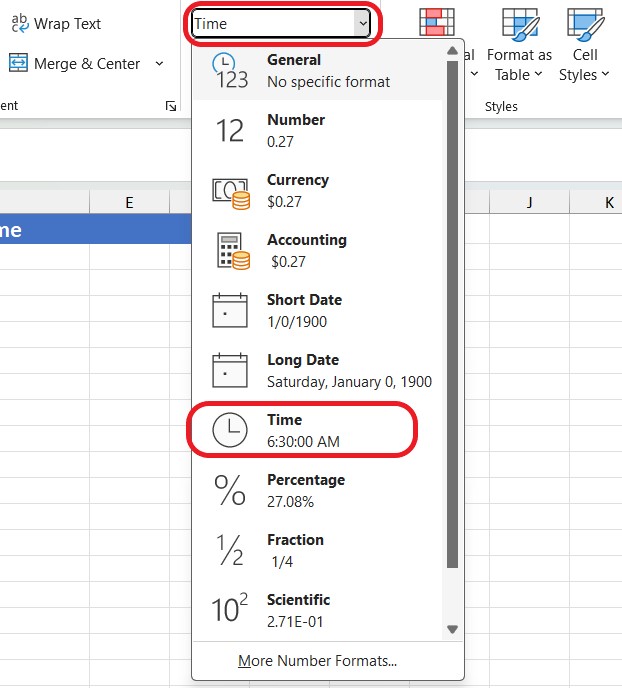
To change the default time format, go to Control Panel and click Region and Language. If your control panel is open in Category View, click Clock, Language, and Region > Region and Language > Change the date, time, or number format.
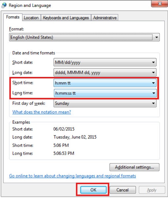
Note: When you want to create a new Excel time format or want to modify the current format, remember that no matter how you choose to display times in a cell, Excel always stores times internally the same way – with decimal places.
5. How to insert time and a timeline in Excel:
There are several ways to insert time into Excel, but which one you use depends on whether you want a fixed time or a changing value (which is automatically updated to show the current time).
5.1 Add to timeline with shortcuts:
If you are looking for a way to insert a timestamp into an Excel cell, i.e. a static value (that does not automatically update even if the spreadsheet is recalculated), use one of the following shortcuts:
- Insert current time, press Ctrl + Shift +;
- Insert the current time: Enter the current date and time, press Ctrl +; to insert a date, then press the Space key , then press Ctrl + Shift +;

5.2 Add current date and current time using NOW function
If your purpose is to insert the current date and time as a dynamic value (that is automatically updated), use the NOW function in Excel.
The formula is as simple as it can be written as follows: (no required arguments)
= NOW ()
When using the NOW function in Excel, there are a few things to keep in mind:
- The NOW function retrieves the time from the computer’s system clock.
- The NOW function is one of the volatile functions in Excel, meaning that cells with this formula will be calculated every time the spreadsheet is reopened or recalculated.
- To force the NOW function to update the returned value, press Shift + F9 to recalculate the current worksheet or F9 to recalculate all open worksheets.
- To get the NOW function to automatically update at certain intervals, add a VBA macro to your spreadsheet, some examples are available here.
5.3 Insert current time as a dynamic value
If you just want to insert the current time into the cell without inserting the date, here are the options for you to refer to:
- Use the formula =NOW(), and then apply the time format in 1 or more cells.
Remember, this will only change the display format, the actual value stored in a cell will still be a decimal number consisting of an integer part representing the date and a decimal part representing the time.
- Use the following formula : =NOW() – INT(NOW())
The INT function is used to round the decimal number returned by NOW() down to the nearest integer. And then you subtract the integer portion representing today’s date to get the decimal portion representing the current time.
Since the formula returns a decimal, you will need to apply a time format to the cells that causes the value to display as a time.
The following screenshot illustrates both formulas. Notice that while the time format values are the same (column C), the actual values stored in the cells (column D) are different – D4 only contains decimals:
5.4 Insert time using TIME function
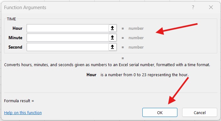
The TIME function in Excel is used to convert a text string representing a time into a decimal number representing the time.
The syntax of the Excel TIME function is very simple:
= TIME (hour,minute,second)
The hour, minute, and second arguments can be entered as numbers from 0 to 3276.
If hour is greater than 23, then it will be divided by 24 and the remainder will be taken as the hour value.
For example, TIME(30, 0, 0) is equivalent to TIME(6,0,0), which is both 0.25 or 6am.
If minute is greater than 59, it is converted to hours and minutes. And if second is greater than 59, it is converted to hours, minutes and seconds.
For example, TIME(0, 930, 0) is converted to TIME(15, 30, 0), which is 0.645833333 or 15:30.
The TIME function is actually useful for combining individual values into a single time value, such as values in other cells or returned by other Excel functions.
6. How to get hours, minutes and seconds from a timestamp
To get each time unit in the timeline, you can use the time formula function as below:
HOUR(serial_number) – returns the hour value of that time, which is an integer ranging from 0 (12:00 AM) to 23 (11:00 PM)
MINUTE(serial_number) – returns the number of minutes in that time value, as an integer with a value between 0 and 59.
SECOND(serial_number ) – returns the number of seconds in that time value, which is an integer with a value between 0 and 59.
In all three formulas, you can enter the time as a string and enclose it in double quotes (for example, “6:00 AM”), or as a fraction (for example, 0.25 means 6:00 AM), or as the result of other Excel functions. You can see some more example formulas below:
- =HOUR(A2) – returns the number of hours in the time frame in cell A1
- =MINUTE(A2) – returns the number of minutes in the time frame in cell A1
- =SECOND(A2) – returns the number of seconds in the timestamp in cell A1
- =HOUR(NOW()) – returns the current time
Now that you understand the time formats and time functions in Excel, it should be much easier for you to manipulate dates and times in your spreadsheets. In the next part of our Excel time tutorial, we will discuss different ways to convert times to numbers. Thanks for reading and hope to see you on our blog next week!
See more at:
